TEXT DATA AND THEIR CORRELATIONS
Correlation analysis helps uncover relationships between variables. When comparing two pieces of text to each other, we aren’t looking for a single “correlation coefficient” in the statistical sense, but rather a similarity measure. These measures tell us how closely related or similar two texts are.
A small sneak peek into this first - Correlation of Text with Numerical Variables
Feature Extraction (Bag-of-Words/TF‑IDF): represent each text (document, sentence, etc.) as a vector of features such as word counts or TF‑IDF scores, each unique word might be a feature dimension transforming the text into a high-dimensional numeric vector.
Derived Numeric Scores: reduce the text to a single meaningful numeric value and then use a standard correlation. A simple example is sentiment analysis where you can assign each text a sentiment score allowing to represent each text with a number.
The Main Concept : Correlation of Text-Text Variables
Now, we have moved to the important section of the article, we will focus on multiple possibilities of exploring the correlations between various text variables.
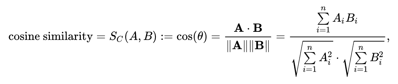
1. Cosine Similarity (Vector-Based Text Correlation):
Cosine similarity is widely used to compare text documents represented as vectors (TF‑IDF vectors, Word2Vec embeddings). It measures the cosine of the angle between two vectors in a multi-dimensional space, If two text vectors point in exactly the same direction, the cosine similarity is 1 (meaning the texts have very similar content in terms of word composition); if they are orthogonal (90° apart), the similarity is 0 (no shared content), and if directly opposite, –1 (though with word count vectors you usually get 0 to 1 because counts are non-negative). Cosine similarity essentially ignores the magnitude of the vectors and focuses on their direction, which is helpful because longer documents might have more words but that doesn’t necessarily mean they are different in topic from a shorter document so, it’s the relative frequency of terms that matters
Formula for cosine similarity
When to Use: Use cosine similarity for any text-to-text comparison where texts are represented as vectors of features (words, terms, n-grams, or even latent semantic vectors). It’s very common in document clustering, duplicate detection (e.g., finding near-duplicate webpages), or recommendation systems (finding similar items based on description text). It’s fast to compute even for high dimensions and works well with sparse data .
Assumptions & Limitations: Cosine similarity assumes the vector representation is meaningful. It doesn’t account for word meaning beyond exact matches (using simple bag-of-words). For example, synonyms are treated as different dimensions. It also doesn’t consider word order or context, just overall frequency. Two sentences with identical words in different order will still get max similarity with cosine. Also, if documents are very short, cosine can be less reliable (since small differences in one word have bigger effect). Pre-processing (TF‑IDF weighting) is important to ensure common but less informative words (“the”, “is”) don’t dominate the similarity. TF‑IDF down-weights common words, which improves cosine similarity’s effectiveness . In summary, cosine is great for comparing content lexical similarity but not deep semantics.
2. Jaccard Similarity (Overlap of Sets):
Jaccard similarity is a simple measure of overlap between two sets. For text, a common approach is to treat each document as a set of words (unique words, ignoring frequency). The Jaccard index between two sets A and B is defined as:
 |
| Jaccard Index formula |
When to Use: Use Jaccard similarity for quick and intuitive comparisons of text where exact word matching is a reasonable gauge of similarity. It’s often used in clustering documents by keywords, or for tasks like near-duplicate detection when small differences in wording should count (plagiarism detection sometimes uses a form of Jaccard on shingled (n-gram) sets). It can also be applied to things like sets of hashtags in social media posts, or any categorical sets.
Assumptions & Limitations: The big limitation is that Jaccard ignores term frequency and meaning. It doesn’t matter if a common word appears 5 times in one doc and 1 time in another, Jaccard only cares that it appears at least once. It also doesn’t account for synonyms or different word forms ( “dog” vs “dogs” count as different unless you preprocess to normalize). Because it’s based on unique set elements, longer documents can seem more similar to each other simply because longer texts tend to contain more common filler words (unless those are filtered). Preprocessing like lowercasing, removing very common words, and perhaps stemming (reducing words to root form) can improve Jaccard comparison. Overall, Jaccard is very simple and is best for cases where vocabulary overlap is the main interest.
3. Semantic Text Similarity with Embeddings:
Modern approaches represent text in vector embeddings that capture semantic meaning. Examples include Word2Vec, GloVe, or contextual embeddings from models like BERT. In these vector spaces, words or sentences with similar meaning end up with vectors that are close together. To quantify similarity between two such embeddings, one typically uses cosine similarity as well (or sometimes Euclidean distance, but cosine is more common for high-dimensional embedding comparison). Essentially, even though this uses cosine mathematically, we treat it as a separate technique because the vector representation is very different from a simple TF‑IDF vector; it encodes semantic relationships learned from large corpora.
If using word embeddings, one can measure similarity between two words by the cosine of their embedding vectors. For example, Word2Vec famously yields that the cosine similarity between “king” and “queen” is high, and between “king” and “apple” is low, reflecting semantic differences. For comparing two longer texts (sentences/documents), one can obtain a sentence embedding or take an average of word embeddings, then compare those. The result is a measure of semantic correlation – do the texts talk about similar things, even if they don’t use the exact same words.
Example: Consider two questions: Q1: “How old is the president of the United States?” and Q2: “What is the age of the US president?”. These two have different wording but identical meaning. A simple Jaccard might be low (they only share “president” and “US/United States” partially), cosine on TF‑IDF might also not be extremely high due to different word forms. But a BERT embedding for each question would yield vectors that are very close, because the model understands they’re paraphrases. The cosine similarity of those embedding vectors would be high (near 1), correctly indicating the texts are essentially the same in content.
When to Use: Use embedding-based similarity when you need to capture semantic relationships, not just exact word overlap. This is common in plagiarism detection beyond copy-paste (ideas expressed differently), semantic search (finding answers that are phrased differently than the query), clustering or matching short texts like FAQ questions with user queries, etc. If you have two pieces of text and want to know if they “mean” the same thing or are on the same topic, word embeddings or sentence embeddings with cosine similarity is a state-of-the-art approach.
Assumptions & Limitations: The power of this approach comes from the underlying model that learned the embeddings. It assumes your text is in the domain/language of the embedding model and that the model has captured the nuances needed. If the text uses jargon or very context-specific language not in the training data, the embeddings might not reflect true similarity. Also, computing good embeddings may require heavy algorithms or pre-trained models. From a correlation perspective, note that cosine similarity on embeddings, while effective, is not as easily interpretable as, say, Pearson’s r on two variables – it’s a measure in a high dimensional semantic space. Another limitation is that comparing long documents by averaging word embeddings can lose word order and context (though advanced models like SBERT produce sentence-level embeddings that do a decent job). Pre-processing typically involves cleaning the text (similar to other methods) and then using a pre-trained model or training one on a large corpus to get the embeddings. After that, computing cosine similarity is straightforward. One should be aware that even embedding similarities can sometimes be fooled, for e.g., a sentence and the same sentence with one crucial word negated (“good” vs “not good”) might end up quite similar unless the model captured the negation effect well.
In Conclusion, Cosine similarity with TF‑IDF is generally more informative than Jaccard for longer texts because it uses frequency and down-weights common terms. Jaccard can be useful for very short text or categorical data like sets of tags. Embedding-based similarity is the most powerful for capturing meaning; however, it’s also the most complex.
NOTE: Correlation is a powerful tool to discover relationships, but it should be complemented with visualization and domain knowledge. And importantly, correlation ≠ causation, it only indicates association.
All the formula images are sourced from the relevant wikipedia pages.


Comments
Post a Comment